Predicting Heart Disease With Advanced Machine Learning: Voting Ensemble Classifier

Heart disease remains one of the leading causes of death globally, making early detection and prediction crucial for saving lives. In this tutorial, we’ll build a machine learning system that can predict the presence of heart disease in patients using an ensemble approach called a voting classifier. This method combines multiple algorithms to create a more accurate and reliable prediction system than any single model could achieve alone.

This guide assumes you have some programming experience but may be new to machine learning. We’ll walk through every step, from data loading and preprocessing to model training, evaluation, and visualization. By the end, you’ll understand not just how to build an ensemble classifier, but why it works and how to interpret its results.

You can download the code from the deepthought.sh code examples repository.

Understanding the Problem and Dataset

Heart disease prediction is a classic binary classification problem where we aim to determine whether a patient has heart disease based on various medical measurements and attributes. For this project, we’ll use the UCI Heart Disease dataset, which contains patient information from multiple medical institutions.

The dataset includes features such as age, sex, chest pain type, resting blood pressure, cholesterol levels, and various other cardiac measurements. Our goal is to predict the target variable, which indicates the presence or absence of heart disease.

Getting the Dataset

The heart disease dataset we’ll be using comes from the UCI Machine Learning Repository and can be downloaded from Kaggle.

This dataset actually combines data from four different medical institutions: Cleveland Clinic Foundation, Hungarian Institute of Cardiology, V.A. Medical Center in Long Beach, and University Hospital in Zurich. Each institution contributed patient records, giving us a diverse and comprehensive dataset for training our model.

Once you download the dataset, you’ll find several files including processed.cleveland.data, processed.va.data, processed.switzerland.data, and reprocessed.hungarian.data. These represent the data from each medical institution, and our preprocessing pipeline will combine them into a unified dataset.

Setting Up the Project Environment

Before diving into the code, let’s establish a clean development environment. This project uses several Python libraries for data manipulation, machine learning, and visualization, so we’ll want to keep everything organized and isolated.

Create a new directory for your project and set up a virtual environment:

mkdir heart-disease-prediction
cd heart-disease-prediction
python -m venv .venv

Activate the virtual environment:

Linux/MacOS:

source .venv/bin/activate

Windows:

.\.venv\Scripts\Activate.ps1

Install the required packages:

pip install scikit-learn pandas numpy matplotlib seaborn joblib

Create the project structure:

mkdir data/raw models reports
touch main.py workflow.py preprocess.py train.py evaluate.py visualize.py

Your project directory should now look like this:

heart-disease-prediction/
├── data/
│   └── raw/                # Place downloaded dataset files here
├── models/                 # Trained models will be saved here
├── reports/                # Generated plots and reports
├── main.py
├── workflow.py
├── preprocess.py
├── train.py
├── evaluate.py
└── visualize.py

Data Loading and Preprocessing Pipeline

The foundation of any successful machine learning project is clean, well-prepared data. Our preprocessing pipeline needs to handle multiple data sources, missing values, feature engineering, and data transformation. Let’s start by examining the preprocess.py module.

Understanding the Data Structure

Each dataset file represents patient records from a different medical institution, and while they follow the same general structure, there are subtle differences in formatting and data quality. The files use different delimiters, and some contain missing values marked with question marks.

Our preprocessing function begins by defining the expected column names for consistency across all datasets:

column_names = [
    'age', 'sex', 'cp', 'trestbps', 'chol', 'fbs', 'restecg',
    'thalach', 'exang', 'oldpeak', 'slope', 'ca', 'thal', 'target'
]

These columns represent various medical measurements and patient characteristics. The target column is what we’re trying to predict, where values greater than zero indicate the presence of heart disease.

The fields contained within the dataset include:

Age: Patient age in years
Sex: Gender (1 = male, 0 = female)
CP: Chest pain type (0-3, representing different angina classifications)
Trestbps: Resting blood pressure in mm Hg
Chol: Serum cholesterol level in mg/dl
FBS: Fasting blood sugar > 120 mg/dl (1 = true, 0 = false)
Restecg: Resting electrocardiographic results (0-2)
Thalach: Maximum heart rate achieved during exercise
Exang: Exercise-induced angina (1 = yes, 0 = no)
Oldpeak: ST depression induced by exercise relative to rest
Slope: Slope of peak exercise ST segment (0-2)
CA: Number of major vessels colored by fluoroscopy (0-3)
Thal: Thallium stress test results (1-3)

Loading Multiple Data Sources

The loading process handles each file individually, accounting for their different formats. Most files use comma separation, but the Hungarian dataset uses whitespace as a delimiter. Our code detects this and adjusts accordingly:

for file_name in data_files:
    file_path = os.path.join(data_dir, file_name)
    
    read_csv_kwargs = {
        'header': None,
        'names': column_names,
        'na_values': '?'
    }
    
    if file_name == 'reprocessed.hungarian.data':
        read_csv_kwargs['delim_whitespace'] = True
    else:
        read_csv_kwargs['sep'] = ','

This approach ensures that all datasets are loaded correctly despite their formatting differences. Missing values marked with question marks are automatically converted to NaN values for proper handling later in the pipeline.

Feature Engineering and Transformation

Once the data is loaded and combined, we perform several important transformations. First, we convert all columns to numeric types, which ensures consistency and allows mathematical operations. The target variable is then binarized, converting any value greater than zero to 1 (indicating heart disease) and zero values to 0 (indicating no heart disease).

An important aspect of our preprocessing is feature engineering. We create squared terms for several key numeric features:

for col in ['age', 'trestbps', 'chol', 'thalach']:
    X[f'{col}_sq'] = X[col]**2

This feature engineering step allows our models to capture non-linear relationships in the data. For example, the relationship between age and heart disease risk might not be purely linear, and including age-squared as a feature gives our models the flexibility to learn these more complex patterns.

Building the Preprocessing Pipeline

The preprocessing pipeline uses scikit-learn’s ColumnTransformer to handle different types of features appropriately. Numeric features receive mean imputation for missing values followed by standardization, while categorical features get mode imputation and one-hot encoding:

numeric_transformer = Pipeline(steps=[
    ('imputer', SimpleImputer(strategy='mean')),
    ('scaler', StandardScaler())
])

categorical_transformer = Pipeline(steps=[
    ('imputer', SimpleImputer(strategy='most_frequent')),
    ('onehot', OneHotEncoder(drop='first', handle_unknown='ignore'))
])

Standardization is particularly important for algorithms like Support Vector Machines and K-Nearest Neighbors, which are sensitive to the scale of input features. One-hot encoding transforms categorical variables into a format that machine learning algorithms can process effectively.

Complete Preprocessing Code

Here’s the complete preprocess.py file that implements all the preprocessing functionality:

import pandas as pd
from sklearn.preprocessing import StandardScaler, OneHotEncoder
from sklearn.compose import ColumnTransformer
from sklearn.impute import SimpleImputer
from sklearn.pipeline import Pipeline
import numpy as np
import os

def load_and_preprocess_data(data_dir: str = 'data/raw'):
    """
    Loads and preprocesses heart disease datasets from multiple sources.
    
    Args:
        data_dir (str): Directory containing the raw data files.
    
    Returns:
        X (pd.DataFrame): Feature matrix after initial engineering.
        y (pd.Series): Binary target vector.
        preprocessor (ColumnTransformer): Scikit-learn transformer for preprocessing.
    """
    
    # Define the expected column names for all datasets
    column_names = [
        'age', 'sex', 'cp', 'trestbps', 'chol', 'fbs', 'restecg',
        'thalach', 'exang', 'oldpeak', 'slope', 'ca', 'thal', 'target'
    ]
    
    # List of all data files to be loaded and combined
    data_files = [
        'processed.cleveland.data',
        'processed.va.data',
        'processed.switzerland.data',
        'reprocessed.hungarian.data'
    ]
    
    df_list = []
    for file_name in data_files:
        file_path = os.path.join(data_dir, file_name)
        
        # Set up arguments for pandas.read_csv
        read_csv_kwargs = {
            'header': None,
            'names': column_names,
            'na_values': '?'
        }
        
        # The Hungarian dataset uses whitespace as a delimiter
        if file_name == 'reprocessed.hungarian.data':
            read_csv_kwargs['delim_whitespace'] = True
        else:
            read_csv_kwargs['sep'] = ','
        
        # Only attempt to load files that exist
        if os.path.exists(file_path):
            df_single = pd.read_csv(file_path, **read_csv_kwargs)
            df_list.append(df_single)
        else:
            print(f"Warning: Data file not found and will be skipped: {file_path}")
    
    # If no files were loaded, raise an error
    if not df_list:
        print(f"Error: No data files found in the specified directory: {data_dir}")
        raise FileNotFoundError(f"No data files found in {data_dir}")
    
    # Concatenate all loaded DataFrames into one
    print(f"Loading and concatenating {len(df_list)} data files...")
    df = pd.concat(df_list, ignore_index=True)
    print(f"Combined dataset has {len(df)} rows.")
    
    # Convert all columns to numeric types
    df = df.apply(pd.to_numeric)
    
    # Binarize the target: 0 = no disease, 1 = presence of disease
    df['target'] = df['target'].apply(lambda x: 1 if x > 0 else 0)
    
    # Separate features and target variable
    X = df.drop('target', axis=1)
    y = df['target']
    
    # Feature engineering: add squared terms for selected numeric features
    for col in ['age', 'trestbps', 'chol', 'thalach']:
        X[f'{col}_sq'] = X[col]**2
    
    # Identify categorical and numeric columns for preprocessing
    categorical_cols = ['sex', 'cp', 'fbs', 'restecg', 'exang', 'slope', 'thal', 'ca']
    numeric_cols = [col for col in X.columns if col not in categorical_cols]
    
    # Define a pipeline for numeric features
    numeric_transformer = Pipeline(steps=[
        ('imputer', SimpleImputer(strategy='mean')),
        ('scaler', StandardScaler())
    ])
    
    # Define a pipeline for categorical features
    categorical_transformer = Pipeline(steps=[
        ('imputer', SimpleImputer(strategy='most_frequent')),
        ('onehot', OneHotEncoder(drop='first', handle_unknown='ignore'))
    ])
    
    # Combine both pipelines into a ColumnTransformer
    preprocessor = ColumnTransformer(transformers=[
        ('num', numeric_transformer, numeric_cols),
        ('cat', categorical_transformer, categorical_cols)
    ], remainder='passthrough')
    
    return X, y, preprocessor

Building the Voting Classifier Ensemble

With our data properly preprocessed, we move to the heart of our approach: the voting classifier ensemble. This technique combines multiple different algorithms to create a single, more accurate predictor. The idea is that different algorithms have different strengths and weaknesses, and by combining them, we can often achieve better performance than any individual model.

Understanding Ensemble Methods

Our voting classifier combines three distinct algorithms, each bringing unique capabilities to the ensemble. Logistic Regression provides a linear baseline that’s interpretable and computationally efficient. K-Nearest Neighbors captures local patterns in the data without making assumptions about the underlying distribution. Support Vector Machines can model complex decision boundaries and work well in high-dimensional spaces.

The ensemble uses “soft voting,” which means instead of simply taking a majority vote of the predictions, it averages the predicted probabilities from each model and selects the class with the highest average probability. This approach typically provides more nuanced and accurate predictions than hard voting.

Constructing the Ensemble

The train.py module implements our ensemble construction and training process. The voting classifier is built by defining a list of base estimators:

estimators = [
    ('lr', LogisticRegression(max_iter=10000, random_state=42)),
    ('knn', KNeighborsClassifier()),
    ('svc', SVC(probability=True, random_state=42))
]

voting_clf = VotingClassifier(estimators=estimators, voting='soft')

Each estimator is given a name and configured with appropriate parameters. The max_iter=10000 parameter for Logistic Regression ensures convergence on our dataset, while probability=True for the SVM enables probability predictions needed for soft voting.

Creating the Complete Pipeline

The final model is a scikit-learn Pipeline that combines preprocessing and classification into a single, coherent workflow:

pipeline = Pipeline([
    ('preprocessor', preprocessor),
    ('classifier', voting_clf)
])

This pipeline approach ensures that all preprocessing steps are applied consistently during both training and inference. When we make predictions on new data, the same scaling, imputation, and encoding transformations are automatically applied.

Complete Training Code

Here’s the complete train.py file that implements the ensemble training:

from sklearn.ensemble import VotingClassifier
from sklearn.linear_model import LogisticRegression
from sklearn.neighbors import KNeighborsClassifier
from sklearn.svm import SVC
from sklearn.pipeline import Pipeline
from joblib import dump
import os

def train_model(X_train, y_train, preprocessor, save_path='models/voting_model.joblib'):
    """
    Builds and trains a full pipeline with a VotingClassifier.
    
    Args:
        X_train: Training feature matrix.
        y_train: Training target vector.
        preprocessor: Preprocessing pipeline for feature transformation.
        save_path (str): File path where the trained model pipeline will be saved.
    
    Returns:
        model: The trained scikit-learn pipeline.
    """
    print("Training a Voting Classifier ensemble...")
    
    # Define the base estimators for the ensemble
    estimators = [
        ('lr', LogisticRegression(max_iter=10000, random_state=42)),
        ('knn', KNeighborsClassifier()),
        ('svc', SVC(probability=True, random_state=42))
    ]
    
    # Create a soft voting classifier
    voting_clf = VotingClassifier(estimators=estimators, voting='soft')
    
    # Build a pipeline that preprocesses data then fits the ensemble
    pipeline = Pipeline([
        ('preprocessor', preprocessor),
        ('classifier', voting_clf)
    ])
    
    # Ensure the directory for saving the model exists
    save_dir = os.path.dirname(save_path)
    if save_dir:
        os.makedirs(save_dir, exist_ok=True)
    
    # Fit the pipeline on the training data
    pipeline.fit(X_train, y_train)
    model = pipeline
    
    # Save the trained pipeline to disk
    dump(model, save_path)
    print(f"Model saved to {save_path}")
    return model

Model Evaluation and Metrics

Evaluating a medical prediction model requires careful consideration of different types of errors and their consequences. In heart disease prediction, both false positives (incorrectly predicting disease) and false negatives (missing actual disease) have important implications, though false negatives are typically considered more serious.

Comprehensive Evaluation Metrics

The evaluate.py module computes a range of classification metrics to give us a complete picture of model performance. The function generates predictions on the test set and uses scikit-learn’s classification_report to compute detailed metrics:

y_pred = model.predict(X_test)
report = classification_report(y_test, y_pred, output_dict=True)

We extract several key metrics from this report, including accuracy, precision, recall, and F1-score, both in macro-averaged and weighted-averaged forms. Weighted recall is particularly important in medical applications because it accounts for class imbalance while emphasizing the model’s ability to correctly identify positive cases.

The evaluation function returns a comprehensive dictionary of metrics:

metrics = {
    'accuracy': accuracy,
    'precision_macro': report['macro avg']['precision'],
    'recall_macro': report['macro avg']['recall'],
    'f1_score_macro': report['macro avg']['f1-score'],
    'precision_weighted': report['weighted avg']['precision'],
    'recall_weighted': weighted_recall,
    'f1_score_weighted': report['weighted avg']['f1-score'],
}

Cross-Validation for Performance Estimation

Beyond simple train-test evaluation, our workflow includes cross-validation to get a more stable estimate of model performance. The workflow.py module performs 5-fold stratified cross-validation using weighted recall as the scoring metric:

self.cross_validation_scores = cross_val_score(
    self.model, self.X_full, self.y_full, 
    cv=StratifiedKFold(n_splits=5, shuffle=True, random_state=42),
    scoring='recall_weighted'
)

Stratified cross-validation ensures that each fold maintains the same proportion of positive and negative cases as the full dataset, providing more reliable performance estimates.

Complete Evaluation Code

Here’s the complete evaluate.py file that implements the evaluation process:

from sklearn.metrics import classification_report


def evaluate_model(model, X_test, y_test, log_results=True):
    """
    Evaluates a trained classification model on a test dataset and logs the results.

    This function generates predictions using the provided model, computes a variety of
    classification metrics, and optionally logs a detailed classification report.
    It is designed to provide both a summary of key metrics for benchmarking and
    a full report for in-depth analysis.

    Args:
        model: Trained scikit-learn compatible classifier with a .predict() method.
        X_test: Features of the test set (array-like or DataFrame).
        y_test: True labels for the test set (array-like or Series).
        log_results (bool): If True, logs the weighted recall and full classification report.

    Returns:
        dict: A dictionary containing accuracy, macro-averaged, and weighted-averaged
              precision, recall, and F1-score metrics.
    """
    # Generate predictions for the test set using the trained model
    y_pred = model.predict(X_test)

    # Compute the classification report as a dictionary for easy metric extraction
    report = classification_report(y_test, y_pred, output_dict=True)
    accuracy = report['accuracy']  # Overall accuracy of the model
    weighted_recall = report['weighted avg']['recall']  # Recall averaged by support (number of true instances for each label)

    if log_results:
        # Log the weighted recall for quick reference
        print(f"Test Set Weighted Recall: {weighted_recall:.4f}")
        # Log the full, human-readable classification report for detailed analysis
        print(f"\nClassification Report:\n{classification_report(y_test, y_pred)}")

    # Collect key metrics for benchmarking and further analysis
    metrics = {
        'accuracy': accuracy,
        'precision_macro': report['macro avg']['precision'],      # Precision averaged equally across classes
        'recall_macro': report['macro avg']['recall'],            # Recall averaged equally across classes
        'f1_score_macro': report['macro avg']['f1-score'],        # F1-score averaged equally across classes
        'precision_weighted': report['weighted avg']['precision'],# Precision averaged by class support
        'recall_weighted': weighted_recall,                       # Recall averaged by class support
        'f1_score_weighted': report['weighted avg']['f1-score'],  # F1-score averaged by class support
    }
    return metrics

Visualization and Model Interpretation

Understanding how well our model performs requires more than just looking at numbers. The visualize.py module provides several plotting functions that help us interpret model behavior and identify potential issues or areas for improvement.

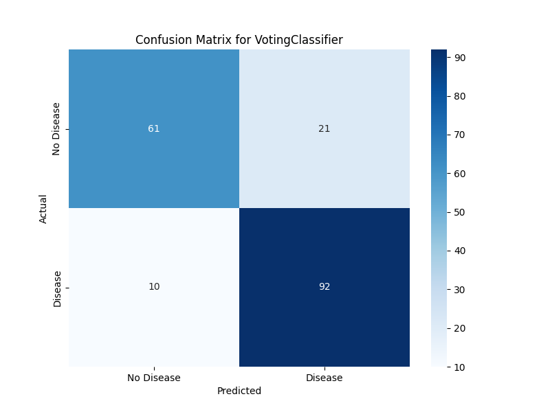
Confusion Matrix Analysis

The confusion matrix provides a detailed breakdown of correct and incorrect predictions. Our plotting function creates a heatmap that makes it easy to see patterns in model errors:

def plot_confusion_matrix(y_true, y_pred, model_name, save_path=None):
    cm = confusion_matrix(y_true, y_pred)
    plt.figure(figsize=(8, 6))
    sns.heatmap(cm, annot=True, fmt='d', cmap='Blues',
                xticklabels=['No Disease', 'Disease'],
                yticklabels=['No Disease', 'Disease'])

The resulting visualization shows true positives, true negatives, false positives, and false negatives in an intuitive format. This helps identify whether the model has particular difficulty with certain types of cases.

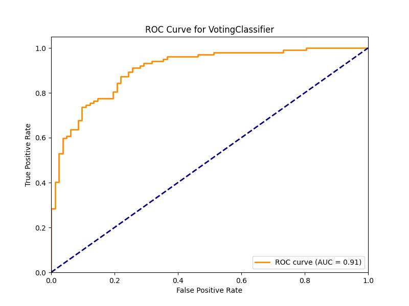
Confusion matrix for heart disease voting classifier

ROC Curve and AUC

The Receiver Operating Characteristic (ROC) curve illustrates the trade-off between sensitivity (true positive rate) and specificity (1 - false positive rate) across different decision thresholds. The Area Under the Curve (AUC) provides a single metric summarizing this trade-off:

def plot_roc_curve(model, X_test, y_test, model_name, save_path=None):
    y_pred_proba = model.predict_proba(X_test)[:, 1]
    fpr, tpr, _ = roc_curve(y_test, y_pred_proba)
    roc_auc = auc(fpr, tpr)

An AUC value closer to 1.0 indicates better model performance, while 0.5 represents random guessing. For medical applications, we typically want AUC values above 0.8 to consider a model clinically useful.

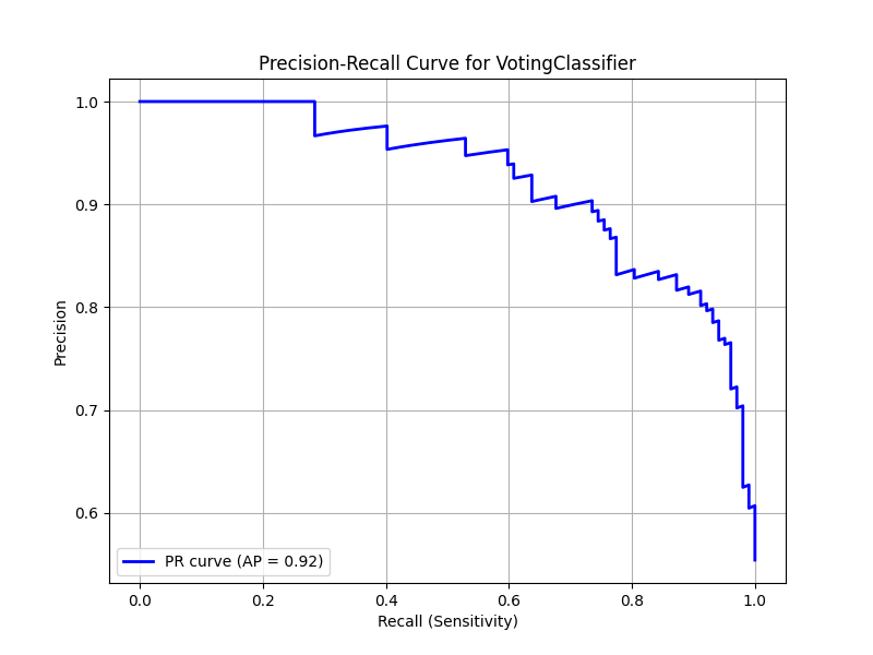
ROC curve for heart disease voting classifier

Precision-Recall Curve

The precision-recall curve is especially valuable for imbalanced datasets or when the cost of false negatives is high. It shows the relationship between precision (positive predictive value) and recall (sensitivity) at different thresholds:

def plot_precision_recall_curve(model, X_test, y_test, model_name, save_path=None):
    y_pred_proba = model.predict_proba(X_test)[:, 1]
    precision, recall, _ = precision_recall_curve(y_test, y_pred_proba)
    avg_precision = average_precision_score(y_test, y_pred_proba)

The average precision score summarizes the precision-recall curve with a single number, similar to how AUC summarizes the ROC curve.

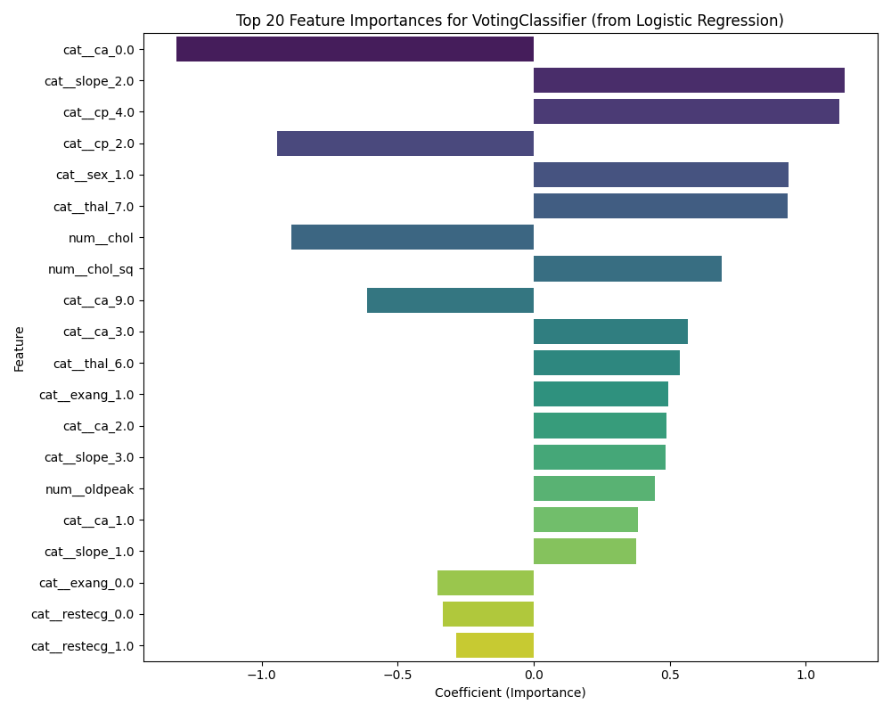
Precision-recall curve for heart disease voting classifier

Feature Importance Analysis

Understanding which features contribute most to predictions helps build trust in the model and can provide clinical insights. Our feature importance plotting function extracts coefficients from the logistic regression component of our ensemble:

def plot_feature_importance(model, preprocessor, model_name, save_path=None):
    feature_names = preprocessor.get_feature_names_out()
    voting_clf = model.named_steps['classifier']
    lr_model = voting_clf.named_estimators_['lr']
    importances = lr_model.coef_[0]

This visualization shows which features have the strongest positive or negative associations with heart disease risk, providing interpretable insights from our ensemble model.

Feature importance for heart disease voting classifier

Complete Visualization Code

Here’s the complete visualize.py file that implements all visualization functions:

import os
import matplotlib.pyplot as plt
import seaborn as sns
import pandas as pd
from sklearn.metrics import confusion_matrix, roc_curve, auc, precision_recall_curve, average_precision_score

def plot_confusion_matrix(y_true, y_pred, model_name, save_path=None):
    """
    Generates and saves a confusion matrix heatmap.
    """
    cm = confusion_matrix(y_true, y_pred)
    plt.figure(figsize=(8, 6))
    sns.heatmap(cm, annot=True, fmt='d', cmap='Blues',
                xticklabels=['No Disease', 'Disease'],
                yticklabels=['No Disease', 'Disease'])
    plt.title(f'Confusion Matrix for {model_name}')
    plt.ylabel('Actual')
    plt.xlabel('Predicted')
    
    if save_path:
        os.makedirs(os.path.dirname(save_path), exist_ok=True)
        plt.savefig(save_path)
        print(f"Saved confusion matrix to {save_path}")
        plt.close()
    else:
        plt.show()

def plot_roc_curve(model, X_test, y_test, model_name, save_path=None):
    """
    Generates and saves a Receiver Operating Characteristic (ROC) curve.
    """
    y_pred_proba = model.predict_proba(X_test)[:, 1]
    fpr, tpr, _ = roc_curve(y_test, y_pred_proba)
    roc_auc = auc(fpr, tpr)
    
    plt.figure(figsize=(8, 6))
    plt.plot(fpr, tpr, color='darkorange', lw=2, label=f'ROC curve (AUC = {roc_auc:.2f})')
    plt.plot([0, 1], [0, 1], color='navy', lw=2, linestyle='--')
    plt.xlim([0.0, 1.0])
    plt.ylim([0.0, 1.05])
    plt.xlabel('False Positive Rate')
    plt.ylabel('True Positive Rate')
    plt.title(f'ROC Curve for {model_name}')
    plt.legend(loc="lower right")
    
    if save_path:
        os.makedirs(os.path.dirname(save_path), exist_ok=True)
        plt.savefig(save_path)
        print(f"Saved ROC curve to {save_path}")
        plt.close()
    else:
        plt.show()

def plot_precision_recall_curve(model, X_test, y_test, model_name, save_path=None):
    """
    Generates and saves a Precision-Recall curve.
    """
    y_pred_proba = model.predict_proba(X_test)[:, 1]
    precision, recall, _ = precision_recall_curve(y_test, y_pred_proba)
    avg_precision = average_precision_score(y_test, y_pred_proba)
    
    plt.figure(figsize=(8, 6))
    plt.plot(recall, precision, color='blue', lw=2, label=f'PR curve (AP = {avg_precision:.2f})')
    plt.xlabel('Recall (Sensitivity)')
    plt.ylabel('Precision')
    plt.title(f'Precision-Recall Curve for {model_name}')
    plt.legend(loc="lower left")
    plt.grid(True)
    
    if save_path:
        os.makedirs(os.path.dirname(save_path), exist_ok=True)
        plt.savefig(save_path)
        print(f"Saved Precision-Recall curve to {save_path}")
        plt.close()
    else:
        plt.show()

def plot_feature_importance(model, preprocessor, model_name, save_path=None):
    """
    Extracts and plots feature importances from the Logistic Regression
    component of the VotingClassifier.
    """
    try:
        # Get feature names from the preprocessor pipeline
        feature_names = preprocessor.get_feature_names_out()
        
        # Extract the logistic regression model and its coefficients
        voting_clf = model.named_steps['classifier']
        lr_model = voting_clf.named_estimators_['lr']
        importances = lr_model.coef_[0]
        
        # Create a DataFrame for easier plotting
        feature_importance_df = pd.DataFrame({
            'feature': feature_names,
            'importance': importances
        }).sort_values(by='importance', key=abs, ascending=False).head(20)
        
        plt.figure(figsize=(10, 8))
        sns.barplot(x='importance', y='feature', data=feature_importance_df, palette='viridis')
        plt.title(f'Top 20 Feature Importances for {model_name} (from Logistic Regression)')
        plt.xlabel('Coefficient (Importance)')
        plt.ylabel('Feature')
        plt.tight_layout()
        
        if save_path:
            os.makedirs(os.path.dirname(save_path), exist_ok=True)
            plt.savefig(save_path)
            print(f"Saved feature importance plot to {save_path}")
            plt.close()
        else:
            plt.show()
    
    except Exception as e:
        print(f"Could not generate feature importance plot: {e}")
        print("This is likely because the model structure is unexpected.")

Orchestrating the Complete Workflow

The PredictionWorkflow class in workflow.py brings all these components together into a cohesive, reproducible pipeline. This class manages the entire process from data loading through final reporting, ensuring that each step is executed in the correct order and that results are properly logged and saved.

Workflow Structure and Organization

The workflow is designed as a sequence of distinct phases, each with clear responsibilities and outputs. The run method orchestrates the entire process:

def run(self):
    print("Starting the prediction workflow...")
    self.load_and_preprocess()
    self.train()
    self.evaluate()
    self.report()
    print("Prediction workflow completed.")

This modular structure makes it easy to debug individual components, modify specific steps, or add new functionality without affecting the rest of the pipeline.

Data Splitting and Validation Strategy

The workflow uses stratified sampling to split the data into training and testing sets, ensuring that both sets have similar distributions of positive and negative cases:

self.X_train, self.X_test, self.y_train, self.y_test = train_test_split(
    self.X_full, self.y_full, test_size=0.2, random_state=42, stratify=self.y_full
)

This approach provides a fair evaluation of model performance and helps ensure that our results will generalize to new, unseen data.

Complete Workflow Code

Here’s the complete workflow.py file that orchestrates the entire pipeline:

import numpy as np
from sklearn.model_selection import cross_val_score, StratifiedKFold, train_test_split
from preprocess import load_and_preprocess_data
from train import train_model
from evaluate import evaluate_model
from visualize import plot_confusion_matrix, plot_roc_curve, plot_precision_recall_curve, plot_feature_importance
import warnings
warnings.filterwarnings('ignore')

class PredictionWorkflow:
    """
    A class to manage the end-to-end prediction workflow.
    """
    
    def __init__(self, model_path='models/voting_classifier_model.joblib',
                confusion_matrix_path='reports/confusion_matrix.png',
                roc_curve_path='reports/roc_curve.png',
                pr_curve_path='reports/precision_recall_curve.png',
                feature_importance_path='reports/feature_importance.png'):
        """
        Initializes the PredictionWorkflow with file paths.
        """
        self.model_path = model_path
        self.confusion_matrix_path = confusion_matrix_path
        self.roc_curve_path = roc_curve_path
        self.pr_curve_path = pr_curve_path
        self.feature_importance_path = feature_importance_path
        self.model = None
        self.preprocessor = None
    
    def run(self):
        """
        Executes the complete prediction workflow.
        """
        print("Starting the prediction workflow...")
        self.load_and_preprocess()
        self.train()
        self.evaluate()
        self.report()
        print("Prediction workflow completed.")
    
    def load_and_preprocess(self):
        """
        Loads and preprocesses the data, splitting it into training and testing sets.
        """
        print("Loading and preprocessing data...")
        X_engineered, y_engineered, self.preprocessor = load_and_preprocess_data()
        self.X_full = X_engineered
        self.y_full = y_engineered
        
        # Stratified split ensures similar class distributions
        self.X_train, self.X_test, self.y_train, self.y_test = train_test_split(
            self.X_full, self.y_full, test_size=0.2, random_state=42, stratify=self.y_full
        )
        print("Data loading and preprocessing complete.")
        print("-" * 50)
    
    def train(self):
        """
        Trains the model using the training data.
        """
        print("Training the model...")
        self.model = train_model(self.X_train, self.y_train, self.preprocessor, save_path=self.model_path)
        print("Model training complete.")
    
    def evaluate(self):
        """
        Evaluates the trained model on the test data and performs cross-validation.
        """
        print("Evaluating the model...")
        self.evaluation_metrics = evaluate_model(self.model, self.X_test, self.y_test)
        
        # Perform 5-fold stratified cross-validation
        self.cross_validation_scores = cross_val_score(
            self.model, self.X_full, self.y_full, 
            cv=StratifiedKFold(n_splits=5, shuffle=True, random_state=42),
            scoring='recall_weighted'
        )
        print("Model evaluation complete.")
        print("-" * 50)
    
    def report(self):
        """
        Generates and saves visualizations and logs evaluation metrics.
        """
        print("Generating and saving reports...")
        
        # Generate predictions for visualization
        y_pred = self.model.predict(self.X_test)
        
        # Plot and save confusion matrix
        plot_confusion_matrix(self.y_test, y_pred,
                              model_name='VotingClassifier',
                              save_path=self.confusion_matrix_path)
        
        # Plot and save ROC curve
        plot_roc_curve(self.model, self.X_test, self.y_test,
                       model_name='VotingClassifier', save_path=self.roc_curve_path)
        
        # Plot and save Precision-Recall curve
        plot_precision_recall_curve(self.model, self.X_test, self.y_test,
                                    model_name='VotingClassifier', save_path=self.pr_curve_path)
        
        # Plot and save feature importance
        plot_feature_importance(self.model, self.model.named_steps['preprocessor'],
                                model_name='VotingClassifier', save_path=self.feature_importance_path)
        
        # Log summary metrics and cross-validation results
        print("*" * 50)
        print("*    Heart Disease Prediction Workflow Report    *")
        print("*" * 50)
        print("Evaluation Metrics:")
        for metric, value in self.evaluation_metrics.items():
            print(f"  {metric}: {value:.4f}")
        print("-" * 50)
        print(f"Cross-validation recall: {self.cross_validation_scores.mean():.4f} ± {self.cross_validation_scores.std():.4f}")
        print("Reporting complete.")

if __name__ == '__main__':
    workflow = PredictionWorkflow()
    workflow.run()

Running the Complete Pipeline

With all components in place, running the entire heart disease prediction workflow is straightforward. The main.py file serves as the entry point and simply instantiates the workflow class and executes it.

Complete Main Script

Here’s the complete main.py file:

from workflow import PredictionWorkflow

def main(): 
    """
    Main function to execute the prediction workflow.
    """
    workflow = PredictionWorkflow()
    workflow.run()

if __name__ == '__main__':
    main()

Before running the pipeline, make sure your project directory is properly set up with the dataset files in the data/raw/ folder. Then execute the main script:

python main.py

Understanding the Output

As the workflow runs, you’ll see progress messages logged to the console, indicating which phase is currently executing. The process typically takes a few minutes to complete, depending on your system specifications and the size of the dataset.

Upon completion, you’ll find several new files in your project directory:

The models/ folder will contain the trained voting classifier pipeline saved as a joblib file. The reports/ folder will have four visualization files: confusion matrix, ROC curve, precision-recall curve, and feature importance plot. These visualizations provide useful insights into model performance and behavior.

The console output will display final evaluation metrics, including accuracy, precision, recall, and F1-scores, as well as cross-validation results that give you confidence in the model’s expected performance on new data.

Interpreting Results and Model Performance

Once your pipeline has completed, take time to examine the generated visualizations and metrics. The confusion matrix will show you exactly how many patients the model correctly and incorrectly classified. Look for patterns: does the model tend to miss more positive cases (false negatives) or incorrectly flag healthy patients (false positives)?

The ROC curve and its associated AUC score provide insight into the model’s discriminative ability across different decision thresholds. An AUC above 0.85 generally indicates good performance for medical prediction tasks, while values above 0.9 suggest excellent performance.

The feature importance plot reveals which patient characteristics most strongly influence the model’s predictions. You might see features like chest pain type, maximum heart rate achieved, or ST depression having high importance, which aligns with clinical knowledge about heart disease risk factors.

Cross-Validation Insights

The cross-validation results give you a sense of how stable your model’s performance is across different subsets of the data. A small standard deviation in cross-validation scores suggests that your model’s performance is consistent and reliable, while large variations might indicate overfitting or sensitivity to particular data patterns.

Extending and Improving the Model

This tutorial provides a solid foundation for heart disease prediction, but there are many ways to extend and improve the system. You might experiment with different algorithms in your ensemble, such as Random Forests or Gradient Boosting machines. Hyperparameter tuning using techniques like Grid Search or Random Search could optimize each model’s performance.

Feature engineering presents another avenue for improvement. You could create interaction terms between features, apply polynomial transformations, or derive new features based on clinical knowledge. For example, calculating ratios between different measurements or creating age-adjusted risk scores might improve predictive performance.

The preprocessing pipeline could also be enhanced with more sophisticated imputation techniques, outlier detection and removal, or feature selection methods that automatically identify the most informative variables.

Advanced Feature Engineering Examples

To give you an example of ways you could apply advanced feature engineering to give your prediction models more data to learn from, see the below code snippet:


    # --- Feature Engineering directly on the DataFrame ---

    # a. Interaction Features: Capture potential nonlinear relationships between features.
    X['age_x_thalach'] = X['age'] * X['thalach']  # Interaction between age and max heart rate.
    X['trestbps_x_chol'] = X['trestbps'] * X['chol']  # Interaction between resting BP and cholesterol.
    X['exang_x_oldpeak'] = X['exang'] * X['oldpeak']  # Interaction between exercise-induced angina and ST depression.

    # b. Ratio Features: Provide normalized measures that may reveal underlying patterns.
    X['oldpeak_div_thalach'] = X['oldpeak'] / (X['thalach'] + 1e-6)  # Avoid division by zero.
    X['trestbps_div_age'] = X['trestbps'] / (X['age'] + 1e-6)

    # c. Log Transformation for skewed features: Reduces skewness and stabilizes variance.
    for col in ['trestbps', 'chol', 'oldpeak']:
        X.loc[X[col] < 0, col] = np.nan  # Negative values are set to NaN as they are not physiologically plausible.
        X[f'{col}_log'] = np.log1p(X[col])  # log1p handles zero and positive values safely.

    # d. Binning for Age: Converts continuous age into categorical bins for potential non-linear effects.
    age_bins = [0, 40, 50, 60, 100]
    age_labels = ['<40', '40-49', '50-59', '60+']
    X['age_binned'] = pd.cut(X['age'], bins=age_bins, labels=age_labels, right=False)     

    # Define categorical columns for preprocessing. Includes both original and engineered categorical features.
    categorical_cols = ['sex', 'cp', 'fbs', 'restecg', 'exang', 'slope', 'thal', 'ca', 'age_binned']
    # All other columns are treated as numeric.
    numeric_cols = [col for col in X.columns if col not in categorical_cols]

Deployment Considerations

For real-world deployment, you’d want to add error handling, input validation, and logging. The model should be wrapped in an API that can receive patient data and return predictions in a standardized format. Consider implementing model monitoring to track performance over time and detect when retraining might be necessary.

See our tutorial series where we build an image classifier and deploy it as an API for inspiration.

Conclusion and Next Steps

Throughout this tutorial, we’ve built a basic machine learning system for heart disease prediction. We started with raw data from multiple medical institutions, created a preprocessing pipeline that handles missing values and feature engineering, built a voting classifier ensemble that combines multiple algorithms, and implemented thorough evaluation and visualization capabilities.

The voting ensemble approach provides several advantages over single models:

improved accuracy through algorithmic diversity
increased reliability through consensus predictions
better generalization to new data.

The techniques and patterns demonstrated here extend far beyond heart disease prediction. The same workflow structure can be applied to other classification problems, the preprocessing pipeline can handle different types of medical data, and the ensemble approach can be adapted with different base algorithms.

As you continue developing machine learning systems, remember that model performance is just one aspect of a successful project. Data quality, reproducible workflows, thorough evaluation, and clear interpretation are equally important for building systems that can be trusted and deployed in real-world applications.

Whether you’re working on medical prediction, financial modeling, or any other classification task, the principles and techniques covered in this tutorial provide a solid foundation for building effective machine learning systems.