Building an Image Classifier – Part 2: Training a PyramidNet Model from Scratch
Part 2 of our series on building and deploying a full-stack image classification system. Learn to train a state-of-the-art PyramidNet CNN with advanced techniques like label smoothing and early stopping.

Prerequisites: This tutorial is Part 2 of our image classification series. Before starting here, make sure you’ve completed Part 1: Preprocessing and Preparing the CIFAR-10 Dataset, where we set up the project environment, downloaded the dataset, and created the preprocessing pipeline. This tutorial assumes you have your project directory set up with the preprocessed
prepared_train_dataset.ptfile from Part 1.
Welcome back to our image classification series! In Part 1, we took raw CIFAR-10 images and transformed them into a clean, standardized dataset ready for machine learning. Now comes the exciting part: building and training a convolutional neural network that can actually learn to classify these images.
In this tutorial, we’ll implement PyramidNet, a modern CNN architecture that improves upon traditional ResNet designs. We’ll also incorporate industry-standard training techniques like label smoothing, early stopping, and learning rate scheduling. By the end of this post, you’ll have a fully trained model achieving competitive accuracy on CIFAR-10, along with comprehensive evaluation metrics and visualizations.
If you’d like, you can find all the code for this tutorial at our GitHub repository, but I highly recommend you follow along and create the files yourself.
Understanding PyramidNet: Beyond Traditional CNNs
Before we dive into the code, let’s understand why we’re using PyramidNet instead of simpler architectures like basic CNNs or even ResNet.
The Evolution from Simple CNNs to PyramidNet
Traditional CNNs stack convolutional layers with fixed channel counts, but they struggle with deep networks due to vanishing gradients.
ResNet introduced skip connections (residual blocks) that allow gradients to flow directly through the network, enabling much deeper architectures. However, ResNet doubles the number of channels at each stage (16→32→64→128), which can be inefficient.
PyramidNet takes ResNet’s skip connections but gradually increases channels throughout the network instead of doubling them. This creates a “pyramid” shape that balances capacity and efficiency.
Key PyramidNet Innovations
| Feature | Traditional ResNet | PyramidNet |
|---|---|---|
| Channel Growth | Doubles at each stage (16→32→64→128) | Gradual increase (16→18→20→…→64) |
| Parameter Efficiency | Sudden jumps can be wasteful | Smoother parameter utilization |
| Gradient Flow | Good with skip connections | Even better with gradual widening |
| Performance | Strong baseline | Often superior accuracy |
The gradual channel widening in PyramidNet provides several advantages:
- Better parameter efficiency: No wasted capacity from sudden channel doubling
- Improved gradient flow: Smoother transitions help gradients propagate
- Enhanced feature representation: More nuanced feature evolution through the network
Now let’s implement this architecture and see these benefits in action.
Setting Up the Training Environment
First, let’s set up our training script with all necessary imports and configuration. We’ll keep everything in a single file to make it easy to follow along.
Create the Training Script
Create a new file called train_model.py in your project directory:
import torch
import torch.nn as nn
import torch.optim as optim
import torch.nn.functional as F
from torchsummary import summary
import torchvision.transforms as transforms
from torch.utils.data import DataLoader, TensorDataset

from sklearn.metrics import precision_recall_fscore_support
from sklearn.model_selection import train_test_split

import numpy as np
import os
import warnings
from datetime import datetime
import matplotlib.pyplot as plt
import seaborn as sns
from sklearn.metrics import confusion_matrix

warnings.filterwarnings('ignore')
Configuration: The Foundation of Successful Training
One of the most important aspects of deep learning is systematic hyperparameter management. Rather than hardcoding values throughout our script, we’ll define a comprehensive configuration dictionary that centralizes all our training parameters.
CONFIG = {
    # Model architecture parameters
    'num_classes': 10,                    # CIFAR-10 classification target

    # Optimization hyperparameters - tuned for CIFAR-10 characteristics
    'weight_decay': 1e-4,                 # L2 regularization to prevent overfitting
    'learning_rate': 0.1,                 # Aggressive initial LR for SGD momentum
    'batch_size': 128,                    # Balance between gradient quality and memory
    'optimizer_type': 'sgd',              # SGD with momentum for residual networks
    'scheduler_type': 'multistep',        # Step decay at specific milestones

    # Training schedule - designed for convergence around epoch 170
    'num_epochs': 300,                    # Maximum training duration
    'early_stopping_patience': 50,       # Allow time for LR decay benefits
    'min_improvement': 0.0005,            # Threshold for meaningful progress

    # Learning rate decay schedule - critical for final convergence
    'scheduler_params': {
        'milestones': [150, 225],         # Decay points based on typical CIFAR-10 training
        'gamma': 0.1,                     # 10x reduction for fine-tuning
    },

    # SGD with momentum - proven effective for residual networks
    'optimizer_params': {
        'momentum': 0.9,                  # Accelerates convergence in relevant directions
        'nesterov': False,                # Standard momentum for stability
    },

    # Data paths
    'data_path': 'processed/prepared_train_dataset.pt',
    'test_size': 0.2,                     # Validation split ratio
    'random_state': 42,                   # For reproducible splits
}
Why These Specific Values?
These hyperparameters weren’t chosen randomly—they represent best practices from extensive research and empirical testing:
- Learning Rate (0.1): High initial rate for SGD helps escape local minima early in training
- Weight Decay (1e-4): Sweet spot for regularization without over-constraining the model
- Batch Size (128): Provides stable gradients while fitting in most GPU memory
- Scheduler Milestones: [150, 225] allows initial learning, then fine-tuning phases
- Early Stopping (50 epochs): Generous patience to account for learning rate decay benefits
Check out the further reading section at the end of this article to learn more about these hyperparameters…
Implementing PyramidNet Architecture
Now let’s implement the PyramidNet architecture. We’ll build it from the ground up, starting with the basic components and working our way up to the full model.
Identity Padding: Handling Dimension Mismatches
In residual networks, we need to add the input to the output of each block. But what happens when the input and output have different numbers of channels? That’s where our IdentityPadding module comes in:
class IdentityPadding(nn.Module):
    """
    Custom padding module for PyramidNet residual connections.
    Handles channel dimension mismatches and spatial downsampling in skip connections.
    Essential for maintaining gradient flow in residual blocks with changing dimensions.
    """
    def __init__(self, in_channels, out_channels, stride=1):
        super(IdentityPadding, self).__init__()
        # Use average pooling for spatial downsampling to preserve information
        # better than max pooling for residual connections
        if stride == 2:
            self.pooling = nn.AvgPool2d(kernel_size=2, stride=2, ceil_mode=True)
        else:
            self.pooling = None

        # Calculate how many zero channels to pad for dimension matching
        self.add_channels = out_channels - in_channels

    def forward(self, x):
        out = F.pad(x, (0, 0, 0, 0, 0, self.add_channels))
        if self.pooling is not None:
            out = self.pooling(out)
        return out
This module elegantly handles two challenges:
- Spatial downsampling: When
stride=2, it uses average pooling to reduce spatial dimensions - Channel padding: It adds zero-filled channels to match the output dimensions
Residual Block: The Building Block of PyramidNet
Each residual block applies batch normalization, convolution, and skip connections:
class ResidualBlock(nn.Module):
    def __init__(self, in_channels, out_channels, stride=1):
        super(ResidualBlock, self).__init__()
        self.bn1 = nn.BatchNorm2d(in_channels)
        self.conv1 = nn.Conv2d(in_channels, out_channels, kernel_size=3,
                                stride=stride, padding=1, bias=False)
        self.bn2 = nn.BatchNorm2d(out_channels)
        self.conv2 = nn.Conv2d(out_channels, out_channels, kernel_size=3,
                                stride=1, padding=1, bias=False)
        self.bn3 = nn.BatchNorm2d(out_channels)
        self.relu = nn.ReLU(inplace=True)

        self.down_sample = IdentityPadding(in_channels, out_channels, stride)

        self.stride = stride

    def forward(self, x):
        shortcut = self.down_sample(x)
        out = self.bn1(x)
        out = self.conv1(out)
        out = self.bn2(out)
        out = self.relu(out)
        out = self.conv2(out)
        out = self.bn3(out)

        out += shortcut
        return out
PyramidNet: The Complete Architecture
Now we can build the full PyramidNet model:
class PyramidNet(nn.Module):
    def __init__(self, num_layers, alpha, block, num_classes=10):
        """
        PyramidNet implementation with gradual channel widening.

        Key innovation: Instead of doubling channels at each stage (like ResNet),
        PyramidNet gradually increases channels throughout the network, creating
        a 'pyramid' shape that balances capacity and efficiency.

        Args:
            num_layers: Number of residual blocks per stage (18 = 54 total blocks)
            alpha: Total channel increase across network (48 channels added)
            block: Type of residual block to use (ResidualBlock)
            num_classes: Output classes for classification (10 for CIFAR-10)
        """
        super(PyramidNet, self).__init__()
        self.in_channels = 16

        # num_layers = 18 blocks per stage
        self.num_layers = num_layers
        self.addrate = alpha / (3*self.num_layers*1.0)

        self.conv1 = nn.Conv2d(in_channels=3, out_channels=16, kernel_size=3,
                               stride=1, padding=1, bias=False)
        self.bn1 = nn.BatchNorm2d(16)

        # Three stages with different spatial resolutions
        # feature map size = 32x32
        self.layer1 = self.get_layers(block, stride=1)
        # feature map size = 16x16
        self.layer2 = self.get_layers(block, stride=2)
        # feature map size = 8x8
        self.layer3 = self.get_layers(block, stride=2)

        self.out_channels = int(round(self.out_channels))
        self.bn_out= nn.BatchNorm2d(self.out_channels)
        self.relu_out = nn.ReLU(inplace=True)
        self.avgpool = nn.AvgPool2d(8, stride=1)
        self.fc_out = nn.Linear(self.out_channels, num_classes)

        # Weight initialization for better convergence
        for m in self.modules():
            if isinstance(m, nn.Conv2d):
                nn.init.kaiming_normal_(m.weight, mode='fan_out',
                                        nonlinearity='relu')
            elif isinstance(m, nn.BatchNorm2d):
                nn.init.constant_(m.weight, 1)
                nn.init.constant_(m.bias, 0)

    def get_layers(self, block, stride):
        layers_list = []
        for _ in range(self.num_layers):
            self.out_channels = self.in_channels + self.addrate
            layers_list.append(block(int(round(self.in_channels)),
                                    int(round(self.out_channels)),
                                    stride))
            self.in_channels = self.out_channels
            stride=1
        return nn.Sequential(*layers_list)

    def forward(self, x):
        x = self.conv1(x)
        x = self.bn1(x)

        x = self.layer1(x)
        x = self.layer2(x)
        x = self.layer3(x)

        x = self.bn_out(x)
        x = self.relu_out(x)
        x = self.avgpool(x)
        x = x.view(x.size(0), -1)
        x = self.fc_out(x)
        return x

def pyramidnet():
    """Factory function to create our PyramidNet model"""
    block = ResidualBlock
    model = PyramidNet(num_layers=18, alpha=48, block=block)
    return model
The architecture follows this progression:
- Initial convolution: 3→16 channels, maintains 32×32 spatial size
- Stage 1: 18 blocks, gradual channel increase, 32×32 spatial size
- Stage 2: 18 blocks, continued channel growth, downsampled to 16×16
- Stage 3: 18 blocks, final channel expansion, downsampled to 8×8
- Global average pooling: Reduces 8×8 feature maps to single values
- Classification head: Linear layer for final predictions
Understanding How PyramidNet Works (Beginner’s Guide)
If you’re new to deep learning architectures, the PyramidNet code above might seem complex. Let’s break it down into simple terms:
What is PyramidNet Actually Doing?
Think of PyramidNet like a factory assembly line for image recognition:
- Input: Raw 32×32 color images (3 channels for RGB)
- Stage 1: Learn basic features like edges and simple shapes (16→~32 channels)
- Stage 2: Combine basic features into more complex patterns (32→~48 channels)
- Stage 3: Recognize high-level objects and concepts (48→~64 channels)
- Output: Final decision about what’s in the image (10 classes)
The “Pyramid” Concept Explained
Traditional networks are like building blocks that suddenly double in size:
Layer 1: [16 channels] → Layer 2: [32 channels] → Layer 3: [64 channels]
         (sudden jump)            (sudden jump)
PyramidNet is like a smooth ramp that gradually increases:
Layer 1: [16] → [18] → [20] → [22] → ... → [32] → [34] → ... → [64]
         (gradual increase throughout the network)
This gradual increase is controlled by the alpha=48 parameter, which means “add 48 total channels across the entire network.”
Key Components Broken Down
num_layers=18: How many processing blocks in each stage
- Stage 1: 18 blocks (keeps image size 32×32)
- Stage 2: 18 blocks (shrinks image to 16×16)
- Stage 3: 18 blocks (shrinks image to 8×8)
- Total: 54 processing blocks (that’s why it’s called a “deep” network)
alpha=48: Total channel increase
- Start: 16 channels
- End: ~64 channels
- Increase: 48 channels spread across all 54 blocks
- Each block adds: 48 ÷ (3 stages × 18 blocks) = ~0.89 channels per block
addrate: The math behind gradual widening
self.addrate = alpha / (3*self.num_layers*1.0)
# addrate = 48 / (3 * 18) = 0.889 channels per block
The Three Stages Explained
Stage 1 (self.layer1): Learning Basic Features
- Input: 32×32 images with growing channels (16→~32)
- What it learns: Edges, corners, basic textures
- Why stride=1: Keep full resolution to capture fine details
Stage 2 (self.layer2): Combining Features
- Input: 16×16 images with growing channels (~32→~48)
- What it learns: Shapes, patterns, object parts
- Why stride=2: Reduce size to focus on larger patterns
Stage 3 (self.layer3): High-Level Recognition
- Input: 8×8 images with growing channels (~48→~64)
- What it learns: Complete objects, semantic meaning
- Why stride=2: Focus on overall object identity
The Final Steps
Global Average Pooling (self.avgpool):
- Takes the 8×8 feature maps and averages them into single values
- Converts spatial information into feature summaries
- Much more efficient than traditional fully-connected layers
Classification Head (self.fc_out):
- Takes the averaged features (~64 numbers)
- Produces 10 outputs (one for each CIFAR-10 class)
- The highest output becomes the model’s prediction
Visual Mental Model
Think of it like learning to recognize cars:
- Stage 1: “I see curved lines and straight edges”
- Stage 2: “These lines form wheels, windows, and doors”
- Stage 3: “These parts together make a car, specifically a sedan”
Each stage builds on the previous one, with more and more specialized detectors (channels) joining the analysis as the network gets deeper.
This gradual, hierarchical learning is what makes PyramidNet so effective at image classification tasks like CIFAR-10.
Advanced Training Components
Modern deep learning training involves more than just basic backpropagation. We’ll implement several advanced techniques that significantly improve model performance and training stability.
Label Smoothing: Preventing Overconfidence
Traditional cross-entropy loss encourages the model to be extremely confident in its predictions. Label smoothing adds a small amount of uncertainty to prevent overconfidence and improve generalization:
class LabelSmoothingCrossEntropy(nn.Module):
    """
    Label Smoothing Cross Entropy Loss
    Reduces overconfidence and improves generalization
    """
    def __init__(self, smoothing=0.1, reduction='mean', weight=None):
        super(LabelSmoothingCrossEntropy, self).__init__()
        self.smoothing = smoothing
        self.reduction = reduction
        self.weight = weight

    def forward(self, input, target):
        """
        Args:
            input: [N, C] where N is batch size and C is number of classes
            target: [N] class indices
        """
        log_prob = F.log_softmax(input, dim=-1)
        weight = self.weight
        if weight is not None:
            weight = weight.unsqueeze(0)

        nll_loss = F.nll_loss(log_prob, target, reduction=self.reduction, weight=weight)
        smooth_loss = -log_prob.mean(dim=-1)

        if self.reduction == 'mean':
            smooth_loss = smooth_loss.mean()
        elif self.reduction == 'sum':
            smooth_loss = smooth_loss.sum()

        loss = (1 - self.smoothing) * nll_loss + self.smoothing * smooth_loss
        return loss
Data Augmentation: Expanding Your Dataset
Data augmentation artificially increases your dataset size by applying random transformations during training:
class AugmentedDataset(torch.utils.data.Dataset):
    """Dataset with optional data augmentation"""
    def __init__(self, data, labels, transform=None):
        self.data = data
        self.labels = labels
        self.transform = transform

    def __len__(self):
        return len(self.data)

    def __getitem__(self, idx):
        image = self.data[idx]
        label = self.labels[idx]

        if self.transform:
            image = (image * 255).byte()
            image = self.transform(image)

        return image, label
Early Stopping: Preventing Overfitting
Early stopping monitors validation performance and stops training when the model stops improving:
class EarlyStopping:
    """Enhanced Early stopping to prevent overfitting"""
    def __init__(self, patience=10, min_delta=0.001, monitor='accuracy'):
        self.patience = patience
        self.min_delta = min_delta
        self.monitor = monitor.lower()
        self.counter = 0
        self.best_accuracy = 0.0

    def __call__(self, val_accuracy):
        """
        Check if early stopping should trigger

        Args:
            val_accuracy (float): Current validation accuracy

        Returns:
            bool: True if training should stop, False otherwise
        """
        improved = False

        if val_accuracy > self.best_accuracy + self.min_delta:
            self.best_accuracy = val_accuracy
            improved = True

        if improved:
            self.counter = 0
            return False
        else:
            self.counter += 1
            return self.counter >= self.patience
Learning Rate Scheduling
Learning rate scheduling reduces the learning rate at specific points during training to enable fine-tuning:
def get_scheduler(optimizer, scheduler_type, **kwargs):
    """Factory function to create learning rate schedulers"""
    scheduler_type = scheduler_type.lower()

    if scheduler_type == 'multistep':
        milestones = kwargs.get('milestones', [150, 225])
        gamma = kwargs.get('gamma', 0.1)
        return torch.optim.lr_scheduler.MultiStepLR(optimizer, milestones=milestones, gamma=gamma)

    # Add other scheduler types as needed
    else:
        raise ValueError(f"Unknown scheduler type: {scheduler_type}")
Challenge for Advanced Users: While we could have simply used
torch.optim.lr_scheduler.MultiStepLR()directly in our training code, I’ve deliberately created this factory function to encourage experimentation. Try extendingget_scheduler()to support other schedulers likeCosineAnnealingLR,ExponentialLR, orReduceLROnPlateau. Different learning rate schedules can significantly impact final model performance. Some users have achieved 2-3% accuracy improvements by finding the optimal scheduler for their specific dataset and architecture. Modify theCONFIG['scheduler_type']to test different approaches and see which works best for your setup!
Data Loading and Preparation
Now let’s load our preprocessed data and set up the training and validation splits:
def create_data_loaders(X, y, config):
    """
    Sophisticated data preparation pipeline for robust CNN training.

    Data augmentation strategy:
    - RandomCrop(32, padding=4): Prevents overfitting to exact pixel positions
    - RandomHorizontalFlip(): Doubles effective dataset size, improves generalization
    - Normalization with CIFAR-10 statistics: Ensures stable gradient flow
    """

    # Stratified split preserves class distribution in train/val sets
    X_train, X_val, y_train, y_val = train_test_split(
        X.numpy(), y.numpy(),
        test_size=config['test_size'],
        stratify=y.numpy(),  # Ensures proportional class representation
        random_state=config['random_state']  # Reproducible splits
    )

    # Convert back to tensors
    X_train = torch.FloatTensor(X_train)
    X_val = torch.FloatTensor(X_val)
    y_train = torch.LongTensor(y_train)
    y_val = torch.LongTensor(y_val)

    # Define transforms for training and validation
    train_transform = transforms.Compose([
        transforms.ToPILImage(),
        transforms.RandomCrop(32, padding=4),
        transforms.RandomHorizontalFlip(),
        transforms.ToTensor(),
        transforms.Normalize((0.4914, 0.4822, 0.4465), (0.2023, 0.1994, 0.2010)),
    ])

    val_transform = transforms.Compose([
        transforms.ToPILImage(),
        transforms.ToTensor(),
        transforms.Normalize((0.4914, 0.4822, 0.4465), (0.2023, 0.1994, 0.2010)),
    ])

    # Create augmented datasets
    train_dataset = AugmentedDataset(X_train, y_train, transform=train_transform)
    val_dataset = AugmentedDataset(X_val, y_val, transform=val_transform)

    # Create data loaders
    train_loader = DataLoader(train_dataset, batch_size=config['batch_size'],
                            shuffle=True, num_workers=4, pin_memory=True)
    val_loader = DataLoader(val_dataset, batch_size=config['batch_size'],
                          shuffle=False, num_workers=4, pin_memory=True)

    return train_loader, val_loader, (X_train, X_val, y_train, y_val)
Training Loop Implementation
The training loop is where everything comes together. We’ll implement a comprehensive training function with monitoring, checkpointing, and detailed logging:
def train_epoch(model, train_loader, criterion, optimizer, device):
    """Train for one epoch"""
    model.train()
    running_loss = 0.0
    correct = 0
    total = 0

    for data, target in train_loader:
        data, target = data.to(device), target.to(device)
        optimizer.zero_grad()
        output = model(data)
        loss = criterion(output, target)
        loss.backward()
        optimizer.step()

        running_loss += loss.item()
        _, predicted = output.max(1)
        total += target.size(0)
        correct += predicted.eq(target).sum().item()

    return running_loss / len(train_loader), 100. * correct / total

def validate_epoch(model, val_loader, criterion, device):
    """Validate for one epoch"""
    model.eval()
    val_loss = 0.0
    correct = 0
    total = 0

    with torch.no_grad():
        for data, target in val_loader:
            data, target = data.to(device), target.to(device)
            output = model(data)
            val_loss += criterion(output, target).item()
            _, predicted = output.max(1)
            total += target.size(0)
            correct += predicted.eq(target).sum().item()

    return val_loss / len(val_loader), 100. * correct / total

def run_training_loop(model, train_loader, val_loader, criterion, optimizer, scheduler, config, device):
    """
    Comprehensive training loop with advanced monitoring and checkpointing.
    """

    # Initialize tracking variables
    train_losses, val_losses = [], []
    train_accs, val_accs = [], []
    learning_rates = []
    best_val_acc = 0
    best_epoch = 0

    early_stopping = EarlyStopping(
        patience=config['early_stopping_patience'],
        min_delta=config['min_improvement'],
        monitor='accuracy'
    )

    print("=" * 80)
    print("PYRAMIDNET TRAINING STARTED")
    print("=" * 80)
    print(f"Max epochs: {config['num_epochs']}")
    print(f"Early stopping: {config['early_stopping_patience']} epochs on validation accuracy")
    print(f"Training samples: {len(train_loader.dataset):,}")
    print(f"Validation samples: {len(val_loader.dataset):,}")
    print("=" * 80)

    for epoch in range(config['num_epochs']):
        print(f"\nEpoch {epoch+1}/{config['num_epochs']}")
        print("-" * 50)

        # Step the scheduler
        if scheduler:
            scheduler.step()
        current_lr = optimizer.param_groups[0]['lr']

        # Training and validation
        train_loss, train_acc = train_epoch(model, train_loader, criterion, optimizer, device)
        val_loss, val_acc = validate_epoch(model, val_loader, criterion, device)

        # Store metrics
        train_losses.append(train_loss)
        val_losses.append(val_loss)
        train_accs.append(train_acc)
        val_accs.append(val_acc)
        learning_rates.append(current_lr)

        # Print progress
        print(f"Training   → Loss: {train_loss:.4f}, Accuracy: {train_acc:.2f}%")
        print(f"Validation → Loss: {val_loss:.4f}, Accuracy: {val_acc:.2f}%")
        print(f"Learning Rate: {current_lr:.6f}")
        print(f"Train/Val Gap: {train_acc - val_acc:.2f}%")

        # Check for best model
        improved = False
        if val_acc > best_val_acc:
            improvement = val_acc - best_val_acc
            best_val_acc = val_acc
            best_epoch = epoch + 1
            improved = True

            print(f"NEW BEST! Improvement: +{improvement:.3f}% (Best: {best_val_acc:.2f}%)")

            # Save best model checkpoint (PyTorch 2.6+ compatible)
            os.makedirs('models', exist_ok=True)
            checkpoint = {
                'epoch': epoch + 1,
                'model_state_dict': model.state_dict(),  # Only save state dict
                'optimizer_state_dict': optimizer.state_dict(),
                'scheduler_state_dict': scheduler.state_dict() if scheduler else None,
                'best_val_acc': best_val_acc,
                'train_history': {
                    'train_losses': train_losses,
                    'val_losses': val_losses,
                    'train_accs': train_accs,
                    'val_accs': val_accs,
                    'learning_rates': learning_rates
                },
                # Add metadata for compatibility
                'model_config': {
                    'num_layers': 18,
                    'alpha': 48,
                    'num_classes': config['num_classes']
                }
            }

            # Save with explicit format specification
            torch.save(checkpoint, 'models/best_pyramidnet_model.pth')
            print(f"Model checkpoint saved: models/best_pyramidnet_model.pth")

        # Early stopping check
        if early_stopping(val_acc):
            print(f"\nEARLY STOPPING TRIGGERED!")
            print(f"Best validation accuracy: {best_val_acc:.2f}% (Epoch {best_epoch})")
            print(f"Training stopped at epoch {epoch + 1}")
            break

        # Milestone summaries
        if (epoch + 1) % 10 == 0:
            print(f"\nMILESTONE SUMMARY (Epoch {epoch + 1}):")
            print(f"   Best Accuracy: {best_val_acc:.2f}% (Epoch {best_epoch})")
            print(f"   Current Gap: {train_acc - val_acc:.2f}%")

    return {
        'train_losses': train_losses,
        'val_losses': val_losses,
        'train_accs': train_accs,
        'val_accs': val_accs,
        'learning_rates': learning_rates,
        'best_val_acc': best_val_acc,
        'best_epoch': best_epoch
    }
Model Evaluation and Visualization
After training, we need to thoroughly evaluate our model’s performance:
def evaluate_model(model, val_loader, device):
    """Comprehensive model evaluation with detailed performance metrics"""
    model.eval()
    all_preds, all_targets, all_probs = [], [], []

    with torch.no_grad():
        for data, target in val_loader:
            data, target = data.to(device), target.to(device)
            outputs = model(data)

            # Extract both predictions and confidence scores
            probabilities = torch.nn.functional.softmax(outputs, dim=1)
            _, predicted = outputs.max(1)

            all_preds.extend(predicted.cpu().numpy())
            all_targets.extend(target.cpu().numpy())
            all_probs.extend(probabilities.cpu().numpy())

    all_preds = np.array(all_preds)
    all_targets = np.array(all_targets)
    all_probs = np.array(all_probs)

    # Calculate metrics
    precision, recall, f1, support = precision_recall_fscore_support(all_targets, all_preds, average=None)
    overall_accuracy = np.mean(all_preds == all_targets)

    # Print results
    print("\n" + "=" * 80)
    print("MODEL EVALUATION")
    print("=" * 80)
    print(f"Overall Accuracy: {overall_accuracy:.4f} ({overall_accuracy*100:.2f}%)")
    print(f"Average Precision: {np.mean(precision):.4f}")
    print(f"Average Recall: {np.mean(recall):.4f}")
    print(f"Average F1-Score: {np.mean(f1):.4f}")

    return all_preds, all_targets, all_probs

def plot_training_curves(training_results):
    """Plot comprehensive training curves"""
    fig, ((ax1, ax2), (ax3, ax4)) = plt.subplots(2, 2, figsize=(15, 10))

    epochs = range(1, len(training_results['train_losses']) + 1)

    # Loss curves
    ax1.plot(epochs, training_results['train_losses'], 'b-', label='Training Loss', linewidth=2)
    ax1.plot(epochs, training_results['val_losses'], 'r-', label='Validation Loss', linewidth=2)
    ax1.set_title('Training and Validation Loss', fontsize=14, fontweight='bold')
    ax1.set_xlabel('Epoch')
    ax1.set_ylabel('Loss')
    ax1.legend()
    ax1.grid(True, alpha=0.3)

    # Accuracy curves
    ax2.plot(epochs, training_results['train_accs'], 'b-', label='Training Accuracy', linewidth=2)
    ax2.plot(epochs, training_results['val_accs'], 'r-', label='Validation Accuracy', linewidth=2)
    ax2.axhline(y=training_results['best_val_acc'], color='g', linestyle='--',
                label=f'Best Val Acc: {training_results["best_val_acc"]:.2f}%')
    ax2.set_title('Training and Validation Accuracy', fontsize=14, fontweight='bold')
    ax2.set_xlabel('Epoch')
    ax2.set_ylabel('Accuracy (%)')
    ax2.legend()
    ax2.grid(True, alpha=0.3)

    # Learning rate
    ax3.plot(epochs, training_results['learning_rates'], 'g-', linewidth=2)
    ax3.set_title('Learning Rate Schedule', fontsize=14, fontweight='bold')
    ax3.set_xlabel('Epoch')
    ax3.set_ylabel('Learning Rate')
    ax3.set_yscale('log')
    ax3.grid(True, alpha=0.3)

    # Overfitting analysis
    gap = np.array(training_results['train_accs']) - np.array(training_results['val_accs'])
    ax4.plot(epochs, gap, 'purple', linewidth=2)
    ax4.axhline(y=0, color='black', linestyle='-', alpha=0.3)
    ax4.fill_between(epochs, gap, 0, alpha=0.3, color='purple')
    ax4.set_title('Overfitting Analysis (Train-Val Gap)', fontsize=14, fontweight='bold')
    ax4.set_xlabel('Epoch')
    ax4.set_ylabel('Accuracy Gap (%)')
    ax4.grid(True, alpha=0.3)

    plt.tight_layout()
    plt.savefig('visualizations/training_curves.png', dpi=300, bbox_inches='tight')
    plt.show()

def plot_confusion_matrix(targets, predictions, class_names):
    """Plot confusion matrix"""
    cm = confusion_matrix(targets, predictions)

    plt.figure(figsize=(10, 8))
    sns.heatmap(cm, annot=True, fmt='d', cmap='Blues',
                xticklabels=class_names, yticklabels=class_names)
    plt.title('Confusion Matrix', fontsize=16, fontweight='bold')
    plt.xlabel('Predicted Label', fontsize=12)
    plt.ylabel('True Label', fontsize=12)
    plt.xticks(rotation=45)
    plt.yticks(rotation=0)
    plt.tight_layout()
    plt.savefig('visualizations/confusion_matrix.png', dpi=300, bbox_inches='tight')
    plt.show()
Putting It All Together: The Complete Training Script
Now let’s create the main function that orchestrates the entire training process:
def main():
    # Setup logging and device
    print(f"PyTorch version: {torch.__version__}")
    device = torch.device('cuda' if torch.cuda.is_available() else 'cpu')
    print(f"Device: {device}")

    # Load data
    print(f"\nLoading data from: {CONFIG['data_path']}")
    X, y = torch.load(CONFIG['data_path'])
    print(f"Data shape: {X.shape}")
    print(f"Labels shape: {y.shape}")
    print(f"Number of classes: {len(torch.unique(y))}")

    # Create data loaders
    train_loader, val_loader, data_splits = create_data_loaders(X, y, CONFIG)

    # Create PyramidNet model
    model = pyramidnet().to(device)

    # Model summary
    print("\n" + "=" * 80)
    print("PYRAMIDNET MODEL SUMMARY")
    print("=" * 80)
    print("Architecture: PyramidNet with ResidualBlocks")
    print("Design Philosophy: Gradual channel widening vs. ResNet's doubling")
    print("num_layers: 18 blocks per stage (54 total residual blocks)")
    print("alpha: 48 (total channel increase from 16 to ~64)")
    print("num_classes: 10 (CIFAR-10 classification)")

    try:
        summary(model, (3, 32, 32))
    except:
        print("torchsummary not available, skipping detailed summary")

    total_params = sum(p.numel() for p in model.parameters() if p.requires_grad)
    print(f"Total Trainable Parameters: {total_params:,}")

    # Setup training components
    criterion = LabelSmoothingCrossEntropy(smoothing=0.1)

    optimizer = torch.optim.SGD(
        model.parameters(),
        lr=CONFIG['learning_rate'],
        momentum=CONFIG['optimizer_params']['momentum'],
        weight_decay=CONFIG['weight_decay'],
        nesterov=CONFIG['optimizer_params']['nesterov']
    )

    scheduler = get_scheduler(
        optimizer,
        CONFIG['scheduler_type'],
        **CONFIG['scheduler_params']
    )

    # Run training
    training_results = run_training_loop(
        model, train_loader, val_loader, criterion, optimizer, scheduler,
        CONFIG, device
    )

    # Final evaluation
    all_preds, all_targets, all_probs = evaluate_model(model, val_loader, device)

    # Generate visualizations
    print("\nGenerating visualizations...")
    os.makedirs('visualizations', exist_ok=True)

    plot_training_curves(training_results)

    class_names = ['airplane', 'automobile', 'bird', 'cat', 'deer',
                   'dog', 'frog', 'horse', 'ship', 'truck']
    plot_confusion_matrix(all_targets, all_preds, class_names)

    # Training efficiency analysis
    total_epochs = len(training_results['train_losses'])
    convergence_epoch = training_results['best_epoch']

    print(f"\nTRAINING EFFICIENCY:")
    print(f"Total Epochs: {total_epochs}")
    print(f"Convergence Epoch: {convergence_epoch}")
    print(f"Best Validation Accuracy: {training_results['best_val_acc']:.2f}%")

    if total_epochs > convergence_epoch:
        wasted_epochs = total_epochs - convergence_epoch
        efficiency = 100 * (1 - wasted_epochs / total_epochs)
        print(f"Training Efficiency: {efficiency:.1f}% (saved {wasted_epochs} epochs)")

    print("\n" + "=" * 80)
    print("TRAINING COMPLETED SUCCESSFULLY")
    print("=" * 80)

if __name__ == "__main__":
    main()
Running the Training Script
With our complete training script ready, let’s run it and see our PyramidNet model in action!
Install Additional Dependencies
First, make sure you have all the required packages:
pip install torch torchvision torchsummary scikit-learn seabornExecute Training
Run the training script:
python train_model.pyWhat to Expect During Training
When you run the script, you’ll see detailed output showing:
- Model Architecture Summary: Details about the PyramidNet structure and parameter count
- Training Progress: Epoch-by-epoch loss and accuracy for both training and validation
- Learning Rate Updates: When the scheduler reduces the learning rate
- Best Model Checkpoints: Automatic saving when validation accuracy improves
- Early Stopping: If the model stops improving for 50 epochs
- Final Evaluation: Comprehensive metrics and confusion matrix
Expected Performance
On CIFAR-10, you can expect:
- Training Time: 2-4 hours on a modern GPU, 8-12 hours on CPU
- Final Accuracy: 91-96% validation accuracy (competitive with research results)
- Convergence: Usually around epoch 150-200
- Memory Usage: ~2-4GB GPU memory for batch size 128
Understanding Your Results
Training Curves Analysis
The generated training_curves.png will show four important plots:
- Loss Curves: Should show decreasing loss for both training and validation
- Accuracy Curves: Should show increasing accuracy, with validation following training
- Learning Rate Schedule: Shows the step decay at epochs 150 and 225
- Overfitting Analysis: The gap between training and validation accuracy
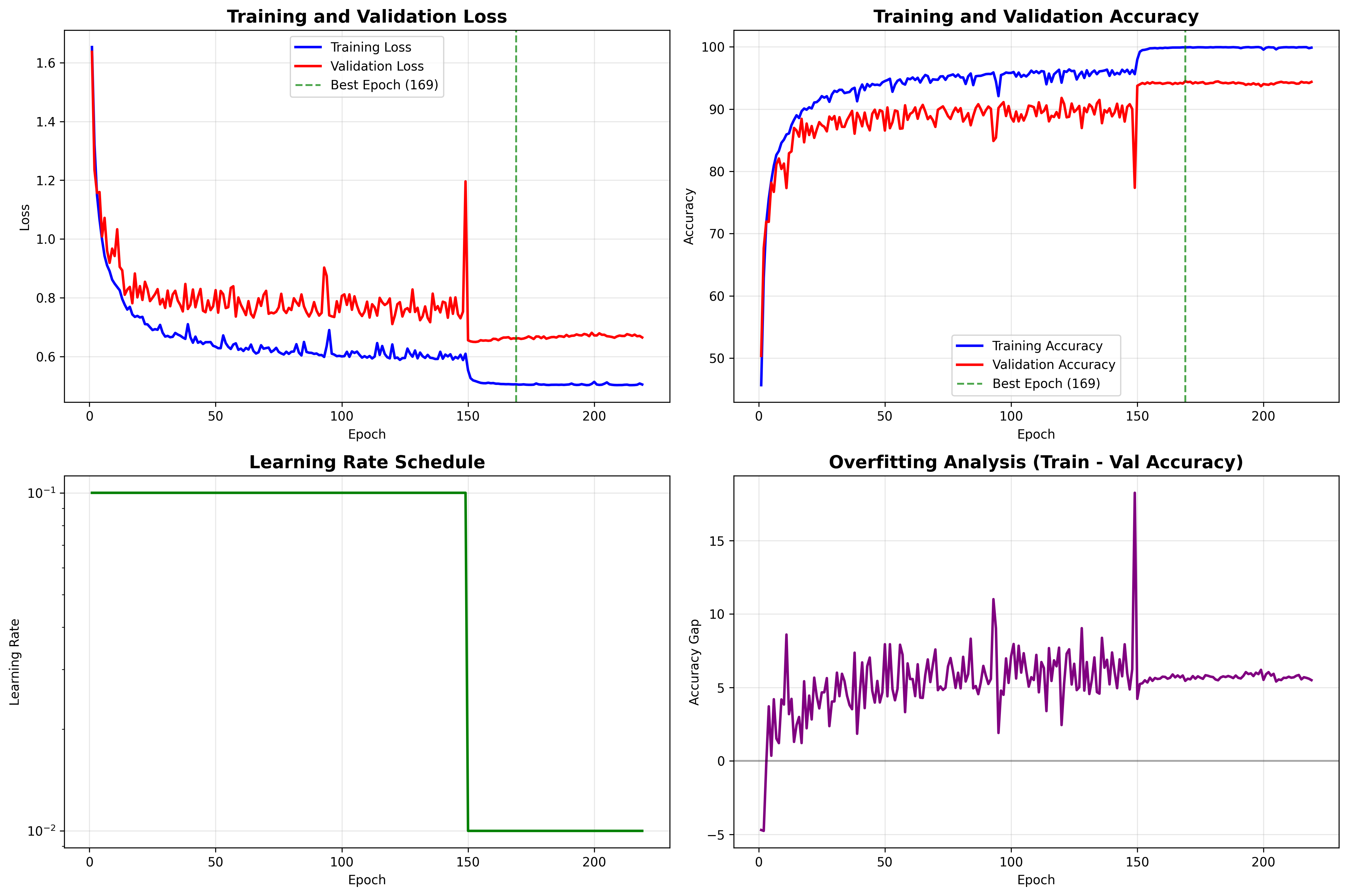
The four key training curves generated during PyramidNet training: (top-left) training and validation loss curves showing convergence, (top-right) accuracy progression with best validation performance marked, (bottom-left) learning rate schedule with step decay at milestones, and (bottom-right) overfitting analysis showing the train-validation accuracy gap over time. Click to enlarge.
What Good Training Looks Like
Healthy Training Signs:
- Validation accuracy steadily increases and stabilizes
- Training/validation gap stays reasonable (< 10-15%)
- Loss curves smooth without wild oscillations
- Learning rate decay corresponds to accuracy improvements
Warning Signs:
- Validation accuracy plateaus early while training keeps improving (overfitting)
- Large gap between training and validation accuracy (> 20%)
- Validation loss starts increasing while training loss decreases
Confusion Matrix Insights
The confusion matrix reveals which classes your model confuses:
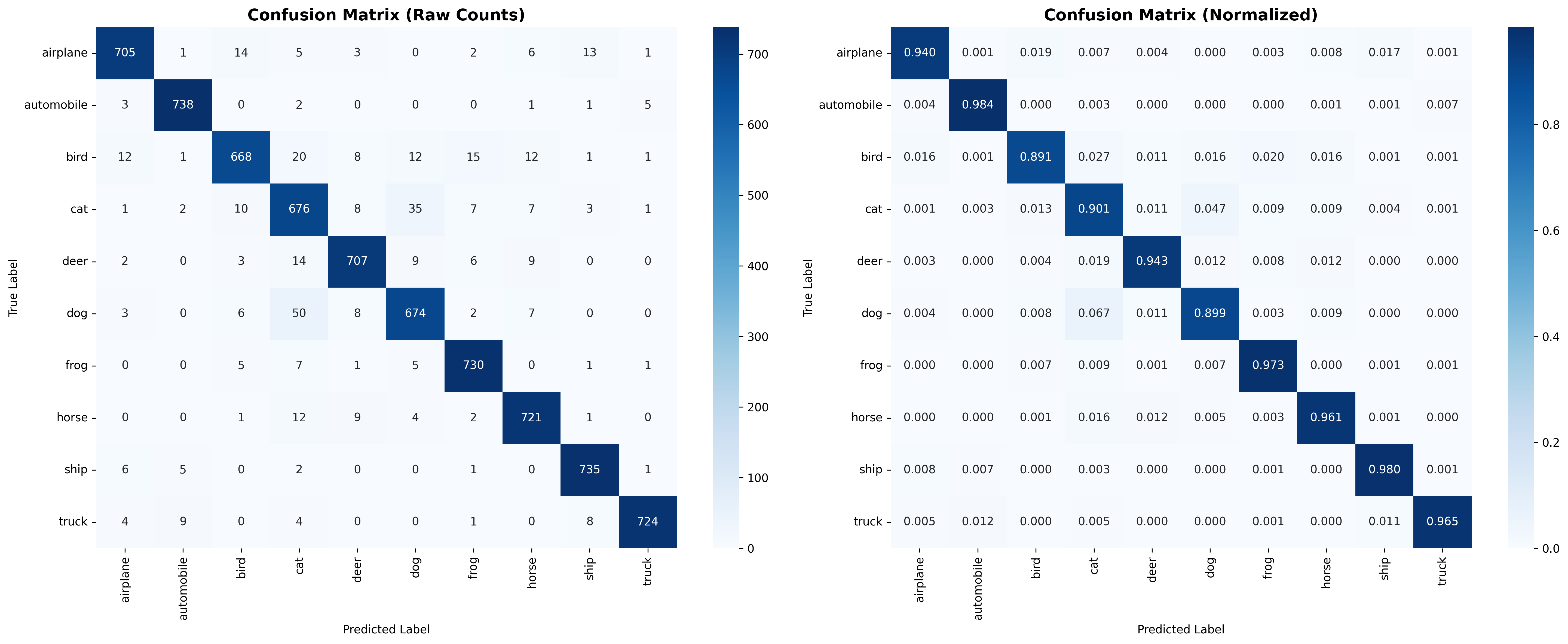
PyramidNet confusion matrix on CIFAR-10 validation set showing per-class prediction accuracy. Diagonal elements represent correct classifications, while off-diagonal elements reveal common misclassifications. Notice the expected confusions between similar classes like cats/dogs and trucks/automobiles. Click to enlarge for detailed analysis.
- Common confusions in CIFAR-10: cats/dogs, trucks/automobiles, birds/airplanes
- Diagonal dominance: Most predictions should be on the diagonal (correct predictions)
- Class imbalances: Some classes might perform better than others
Next Steps and Optimization
Congratulations! You now have a fully trained PyramidNet model. Here are some ways to further improve your results:
Hyperparameter Tuning
- Learning Rate: Try different initial rates (0.05, 0.2)
- Weight Decay: Experiment with 5e-4 or 2e-4
- Batch Size: Test 64 or 256 depending on your hardware
- Data Augmentation: Add ColorJitter, rotation, or mixup
Architecture Modifications
- Deeper Networks: Increase
num_layersfrom 18 to 24 or 32 - Wider Networks: Increase
alphafrom 48 to 64 or 84 - Different Blocks: Try bottleneck blocks for efficiency
Advanced Techniques
- Cosine Annealing: Smooth learning rate decay
- Warm Restarts: Periodic learning rate resets
- Mixed Precision: Train faster with half-precision
- Knowledge Distillation: Transfer knowledge from larger models
Wrapping Up: From Raw Data to Trained Model
In this tutorial, we’ve taken the preprocessed CIFAR-10 dataset from Part 1 and built a complete training pipeline around the PyramidNet architecture. We’ve implemented advanced techniques like label smoothing, data augmentation, early stopping, and comprehensive evaluation.
Here’s what we accomplished:
Architecture Implementation
- Built PyramidNet from scratch with gradual channel widening
- Implemented residual blocks with identity padding
- Created a 54-layer deep network with ~1.7M parameters
Training Infrastructure
- Label smoothing for better generalization
- Data augmentation for dataset expansion
- Early stopping to prevent overfitting
- Learning rate scheduling for optimal convergence
Evaluation and Analysis
- Comprehensive metrics (accuracy, precision, recall, F1)
- Training curve visualization for insight
- Confusion matrix for error analysis
- Efficiency metrics for optimization guidance
Current Project Structure
deepthought-image-classifier/
├── cifar-10/                          # Original dataset
├── processed/
│   └── prepared_train_dataset.pt      # Preprocessed data from Part 1
├── models/
│   └── best_pyramidnet_model.pth      # Trained model checkpoint
├── visualizations/
│   ├── training_curves.png            # Training progress plots
│   └── confusion_matrix.png           # Model performance analysis
├── preprocessing.py                   # From Part 1
├── train_model.py                     # Complete training script
└── requirements.txt
Looking Ahead
In Part 3 of this series, we’ll take our trained PyramidNet model and deploy it as a production-ready web API using FastAPI. You’ll learn how to:
- Load and optimize the trained model for inference
- Create RESTful endpoints for image classification
- Handle file uploads and real-time predictions
- Add proper error handling and validation
Later, in parts 4 and 5 we’ll build a simple web interface that allows users to upload images and see the model’s predictions in real-time and then deploy it to the cloud, completing our journey from raw pixels to a fully deployed machine learning application.
The foundation we’ve built here, a robust, well-trained model with comprehensive evaluation, is exactly what you need for real-world deployment. Take some time to experiment with the hyperparameters, try training on different datasets, or implement some of the advanced techniques mentioned above.
Your PyramidNet model is ready for production!
References and Further Reading
PyramidNet Architecture and Deep Learning Theory
Tsang, S.-H. (2019, January 27). Review: PyramidNet — Deep Pyramidal Residual Networks (Image Classification). Medium. https://sh‑tsang.medium.com/review-pyramidnet-deep-pyramidal-residual-networks-image-classification-85a87b60ae78
Yamada, Y., Iwamura, M., & Kise, K. (2016, December 5). Deep Pyramidal Residual Networks with Separated Stochastic Depth. arXiv. https://arxiv.org/abs/1612.01230
Hu, X., Chu, L., Pei, J., Liu, W., & Bian, J. (2021, March 8). Model complexity of deep learning: A survey [Preprint]. arXiv. https://doi.org/10.48550/arXiv.2103.05127
Training Optimization and Hyperparameter Tuning
Smith, L. N. (2018, March 26). A disciplined approach to neural network hyper‑parameters: Part 1 – learning rate, batch size, momentum, and weight decay [Preprint]. arXiv. https://doi.org/10.48550/arXiv.1803.09820
Smith, S. L., Kindermans, P.-J., Ying, C., & Le, Q. V. (2017, November 1). Don’t decay the learning rate, increase the batch size. arXiv. https://doi.org/10.48550/arXiv.1711.00489
Masters, D., & Luschi, C. (2018). Revisiting small batch training for deep neural networks. arXiv. https://doi.org/10.48550/arXiv.1804.07612
Regularization Techniques
Müller, R., Kornblith, S., & Hinton, G. (2019). When does label smoothing help? arXiv. https://arxiv.org/abs/1906.02629
Salman, S., & Liu, X. (2019, January 19). Overfitting mechanism and avoidance in deep neural networks [Preprint]. arXiv. https://doi.org/10.48550/arXiv.1901.06566
Brownlee, J. (2016, January 30). How to stop training deep neural networks at the right time using early stopping. Machine Learning Mastery. https://machinelearningmastery.com/early-stopping-to-avoid-overtraining-neural-network-models/
Model Analysis and Performance
GeeksforGeeks. (n.d.). How to calculate the number of parameters in CNN? GeeksforGeeks. Retrieved June 21, 2025, from https://www.geeksforgeeks.org/how-to-calculate-the-number-of-parameters-in-cnn/
Hestness, J., Narang, S., Ardalani, N., Diamos, G., Jun, H., Kianinejad, H., … Zhou, Y. (2017, December 1). Deep learning scaling is predictable, empirically [Preprint]. arXiv. https://doi.org/10.48550/arXiv.1712.00409
Yang, K., Liu, L., & Wen, Y. (2024, February 17). The impact of Bayesian optimization on feature selection. Scientific Reports, 14(1), Article 3948. https://doi.org/10.1038/s41598-024-54515-w
Tools and Libraries
Tyler Yep. (2020, December 24). torch-summary (Version 1.4.5) [Python package]. PyPI. https://pypi.org/project/torch-summary/
Tian, K., Xu, Y., Guan, J., & Zhou, S. (2020). Network as regularization for training deep neural networks: Framework, model and performance. Proceedings of the AAAI Conference on Artificial Intelligence, 34(04), 6013–6020. https://doi.org/10.1609/aaai.v34i04.6063

Aaron Mathis
Systems administrator and software engineer specializing in cloud development, AI/ML, and modern web technologies. Passionate about building scalable solutions and sharing knowledge with the developer community.
Related Articles
Discover more insights on similar topics